The Excel ISERR function lets you check whether the given cell contains an error or not. It returns TRUE or FALSE as the output:
- TRUE when the given cell contains an error (except #N/A)
- FALSE when it does not contain an error
The function can identify #VALUE!, #REF!, #DIV/0!, #NUM!, #NAME?, #NULL!, #CALC!, and #SPILL! errors in Excel.
For example, consider the following table, which includes numbers, text strings, and multiple errors.
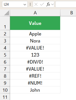

Our task is to identify cells with errors.
Here is the formula:
=ISERR(A2)Where cell A2 holds the first value to be checked for an error or not.
The results are displayed in the following GIF.

Here, I am using conditional formatting to highlight the cells. This helps us visually analyze the cells that include the errors.
Syntax
The ISERR is a simple function with the following syntax. It is mostly combined with the IF function to catch an error and display a custom message.
=ISERR(value)Where the value argument needs to be replaced with a cell reference, a direct value, or the result of another formula.
Important Notes:
- The function is not compatible with the #N/A error
- It returns FALSE for #N/A, valid results, and blank cells
- It can be combined with the lookup functions to catch most errors
How to use the ISERR Function in Excel
Download the example spreadsheet used to demonstrate the ISERR function in the upcoming section. Practice is the key to success!
Example 1: ISERR Function Basics
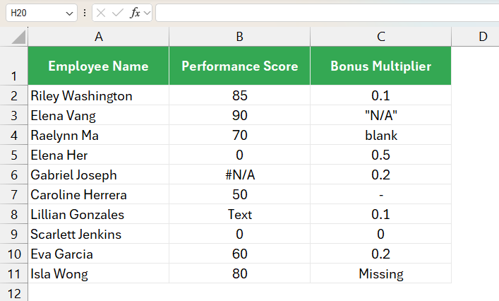
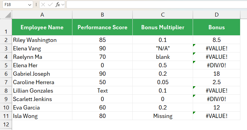
Suppose that you are an HR Manager. You need to calculate the monthly bonus for your company’s sales reps using the following formula:
Bonus = Performance Score x Bonus Multiplier
The sales manager already mentioned the performance score and bonus multiplier in the table. Your task is to find the bonus only.

After using the formula, Excel returned the following errors.


These errors are due to the incorrect entries in the Performance Score and Bonus Multiplier columns.
Let us find the errors in the calculations.
Here are the steps:
- Add a new column
- Select the first cell E2
- Type =ISERR
- Choose the first option from the popup
- Specify the cell reference D2
- Close the bracket using )
- Hit the Enter key

Our formula is as follows:
=ISERR(D2)Where cell D2 contains the bonus for the first employee. The contents of this cell need to be checked if error or not.
The outputs are displayed in the following image.
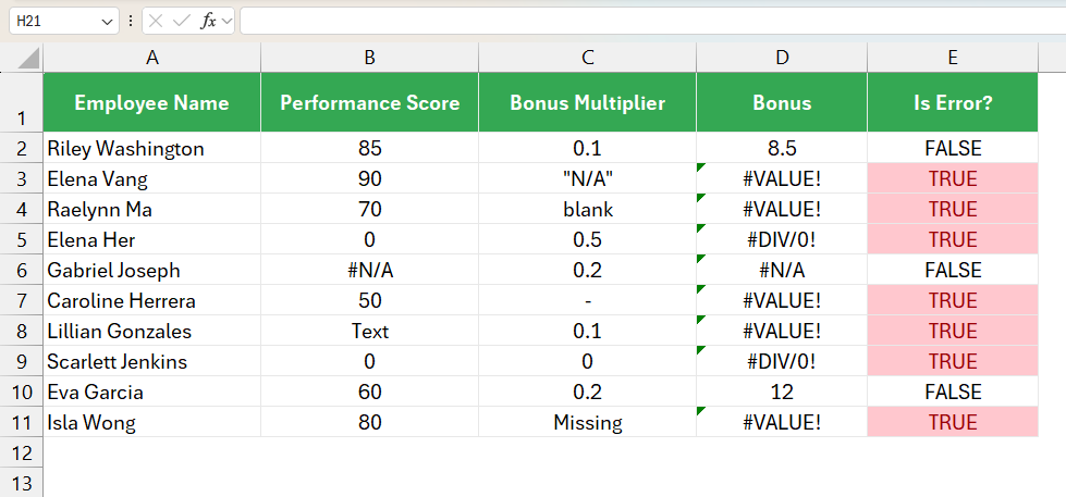

You can use Excel’s Conditional Formatting feature to highlight the errors shown in the above image.
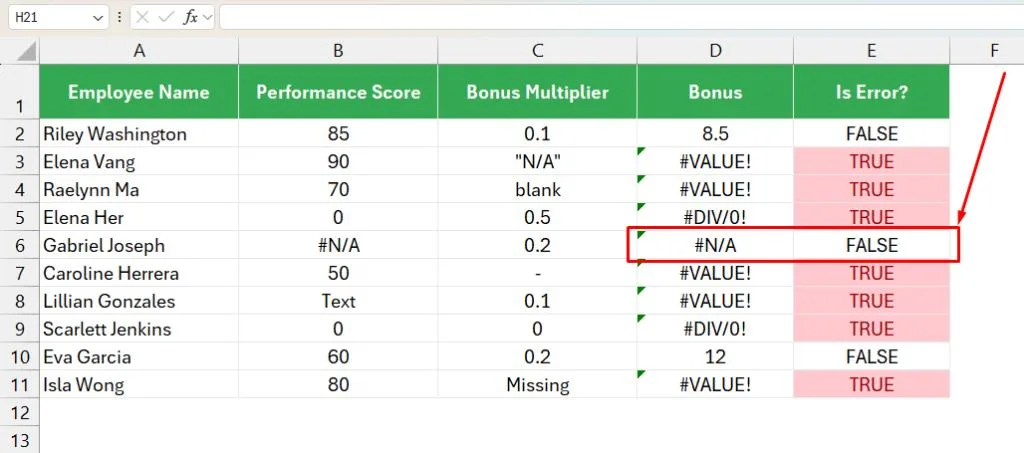
If you have noticed, the ISERR function didn’t catch the #N/A error in the above table. Refer to the following image.

Example 2: Count the errors across the given Array or Range
Let us consider the same scenario as example 1.


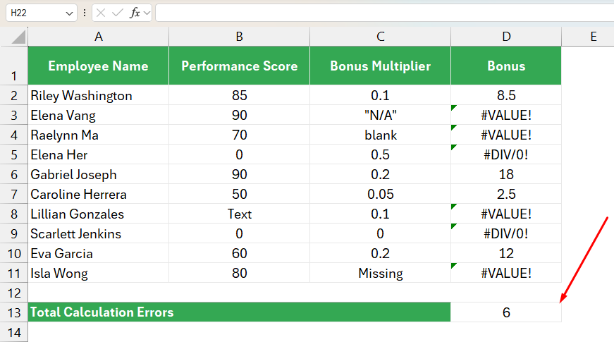
Here, we are calculating bonuses based on performance score and a set bonus multiplier for each employee. As you can see, there are incorrect entries in the Performance Score and Bonus Multiplier columns due to a few mistakes. As a result, the calculation in column D resulted in #VALUE and #DIV/0!
Now, our task is to count the total errors in the above table.
Here are the steps,
- Select the desired cell
- Type =SUM
- Choose the first option from the popup
- Specify —
- Type ISERR
(As the ISERR is a built-in function in Excel, you will see the following popup) - Double-click the ISERR command from the list
- Specify the cell range D2:D11
- Complete the bracket for the ISERR function using )
- Complete the bracket for the SUM function using )
- Hit the Enter key


Our formula would be as follows:
=SUM(--ISERR(D2:D11))Where,
- D2:D11 is the range that includes errors
- ISERR(D2:D11) is the formula applied to each cell in the given array or range to check if it contains an error
- — is the double unary operator which converts Boolean values (TRUE or FALSE) into numbers (1 or 0)
- The SUM function adds all the results obtained by the –ISERR(D2:D11) formula
The results are displayed in the following image.

Example 3: Highlight the Cells with error across the given Array or Range
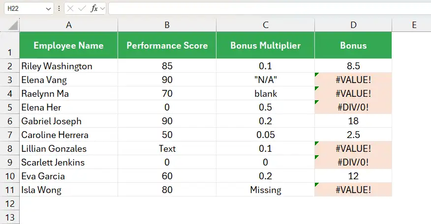
Here as well, we will consider the same scenario. Now, instead of counting the errors, we will highlight them using the conditional formatting feature in Excel.

While calculating the bonus based on performance score and a set bonus multiplier for each sales rep, the formula in column D resulted in #VALUE and #DIV/0!
Our task is to highlight those errors.
Here are the steps:
- Select the entire range
- Hover over the main menu
- Click the Home tab from the ribbon
- Click the Conditional Formatting icon as shown below
- Choose the New Rule option
- You will see the following popup
- Choose the Use a formula to determine which cells to format option
- Enter the formula =ISERR(D2) as shown below
- Click the Format button
- You will see the following popup
- Choose the desired color
- Click the OK button to close the popup
- You will be redirected to the conditional formatting dialog box as shown below
- Click the OK button


When entering the ISERR formula to highlight the first cell, make sure to specify the first cell instead of the entire range.
The results are displayed in the following image.

Takeaway
ISERR is one of the simple functions in Excel that helps you validate the contents of the given cells. You can create complex formulas by combining the ISERR with the IF function to automate various data analysis and management tasks.
I hope this article taught you all the bells and whistles of the ISERR function. Please comment below if you are stuck or encounter any particular error while using the ISERR function. I will answer your questions as soon as possible.
Additional Resources:
- Learn All Excel Information Functions (With Examples)
- IFNA Function in Excel
- ISERROR Function in Excel
- ISTEXT Function in Excel
- IFERROR Function in Excel
- IF Function in Excel
- SEARCH Function in Excel
- Guide to Conditional Formatting in Excel
- SUM Function in Excel
- SUMPRODUCT Function in Excel
Get an Office 365 Subscription to Access all the powerful Functions and Tools in Excel.