The Excel ISNA function lets you check whether the given cell contains a #N/A error or not. It returns TRUE or FALSE as the output:
- TRUE when the given cell contains a #N/A error
- FALSE when it does not contain a #N/A error
The #N/A error is displayed when Excel cannot find what it is looking for across the given array or range.
For example, suppose that you manage a store. You recently received last month’s sales report. Refer to the following image.


You prepared a separate table to determine the sales of your shop’s best-selling products, as shown in the following image. You are using the VLOOKUP function to fetch the sales from the original table.
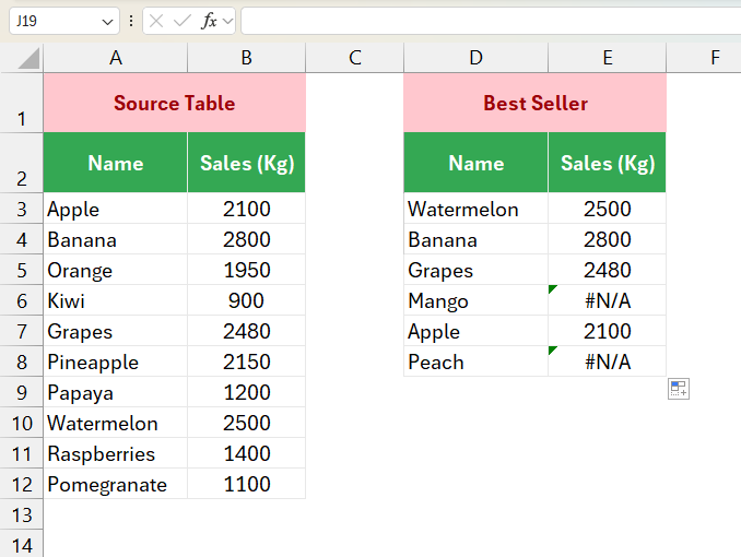

For a few products, the VLOOKUP formula returned a #N/A error. This is because a few best-selling products are seasonal, and their stock was zero in the previous month.
Now, let’s combine the ISNA and IF with the VLOOKUP function to get rid of those #N/A errors.
Our formula would be as follows:
=IF(ISNA(VLOOKUP(D3, A:B, 2, 0)), "Seasonal", VLOOKUP(D3,A:B,2,0))Where,
- VLOOKUP(D3, A:B, 2, 0) is the formula to fetch the sales of the first best-selling product
- ISNA(VLOOKUP(D3, A:B, 2, 0)) is the formula (expression) for the IF function to identify if the given product exists in the source table or not
- Seasonal is the desired output if the formula to fetch the sales cannot find the given product in the source table and returns a #N/A error
The results are displayed in the following GIF.

Here, I am using conditional formatting to highlight the cells. This helps us analyze the seasonal products visually.
Syntax
The ISNA is a simple function with the following syntax. It is mostly combined with other functions like IF and VLOOKUP to catch a #N/A error and display a custom message.
=ISNA(value)Where the value argument needs to be replaced with a cell reference, a direct value, or the result of another formula.
Important Notes:
- The function is compatible with the #N/A error only
- It is mostly combined with the lookup functions like VLOOKUP, HLOOKUP, and MATCH to catch the #N/A error
How to use the ISNA Function in Excel
Download the example spreadsheet used to demonstrate the ISNA function in the upcoming section. Practice is the key to success!
Example 1: ISNA Function Basics
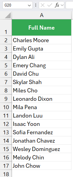
Suppose that you are a teacher. You have two lists as follows:
- The first one includes students who attended your summer webinar
- The second one consists of students who enrolled in your summer learning program
Your task is to identify the students who attended your webinar but didn’t enroll for the summer learning program.
Refer to the following image,


Let us identify the students who attended the webinar but didn’t enroll for the summer learning program by combining the ISNA with the IF and MATCH functions in Excel.
Here are the steps,
- Select the cell B2
- Type =IF
- Choose the first option from the popup
- Type ISNA
(As the ISNA is a built-in function in Excel, you will see the following popup) - Double-click the ISNA command from the list
- Type the formula MATCH(A3, E:E, 0)
- Complete the bracket for the ISNA Function using )
- Type , to move to the next argument of the IF function
- Specify “No”
(Make sure to use the double quotation marks) - Type ,
- Specify “Yes”
(Make sure to use the double quotation marks) - Complete the bracket for the IF function using )
- Hit the Enter key


Our formula is as follows:
=IF(ISNA(MATCH(A3, E:E, 0)), "No", "Yes")Where,
- MATCH(A3, E:E, 0) is the formula to search for the students (who enrolled for the summer learning program) within the webinar attendance list
- ISNA(MATCH(A3, E:E, 0)) is the formula (or expression for the IF function) to find the students who attended the webinar but didn’t join the summer learning program
- No is the desired output if the given student didn’t enroll for the summer program
- Yes is the desired output if the student is enrolled in the summer program
The outputs are displayed in the following image.


You can use Excel’s Conditional Formatting feature to highlight the students who didn’t enroll in the summer learning program.
Example 2: Count the #N/A errors across the given Array or Range
Suppose you are an HR Manager who hired 15 new people to join your company’s sales team. Refer to the following image.

You have received a file for the Sales Manager, which includes salaries for these new team members.
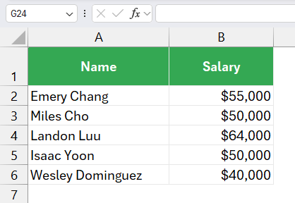

The file includes salaries for a few of the newly hired people.
Now, your task is to identify the people whose salaries have not yet been finalized. We will send this file back to the Sales Manager.
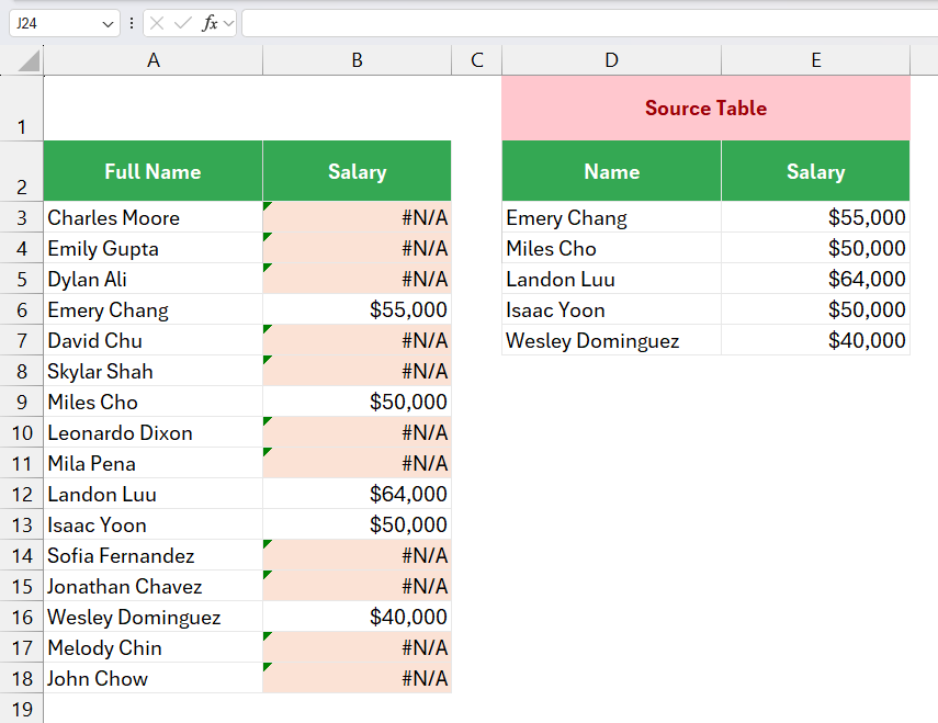
We will use the VLOOKUP function to get this job done. Our formula would be as follows:
=VLOOKUP(A3, D:E, 2, 0)Where,
- A3 includes the first employee’s name who is hired in the sales team
- D:E is the array where the function will search for the employee name
- 2 is the column index number from which the corresponding salary will be returned if the function finds the given name within the source table
- 0 tells the function to look for an exact match
Refer to the following GIF.

As you can see in the following image, the VLOOKUP function returned a #N/A error for the employees whose salaries have not yet been finalized.
Let’s count the total number of employees with #N/A error. For this purpose, we will combine the SUM and ISNA functions with the Double Unary Operator (–) in Excel.
Here are the steps,
- Select the desired cell
- Type =SUM
- Choose the first option from the pop-up
- Type —
- Next, type ISNA
(As the ISNA is a built-in function in Excel, you will see the following popup) - Double-click the ISNA command from the list
- Specify the range Specify the range B3:B18
- Complete the bracket for the ISNA function using )
- Complete the bracket for the SUM function using )
- Hit the Enter key


Our final formula would be as follows:
=SUM(--ISNA(B3:B18))Where,
- B3:B18 is the range that includes salaries
- ISNA(B3:B18) is the formula applied to each cell in the given array or range to check if it contains a #N/A error
- — is the double unary operator which converts Boolean values (TRUE or FALSE) into numbers (1 or 0)
- The SUM function adds all the results obtained by the –ISNA(B3:B18) formula
The results are displayed in the following image.


Example 3: Highlight the Cells with #N/A error across the given Array or Range
We will consider the same scenario as before.


We have the above data, which includes newly hired employees and their salaries. As we can see, a few #N/A errors were returned by the VLOOKUP function while fetching the salaries from the source table.
Now, our task is to highlight the cells that include #N/A errors.
We will use the Conditional Formatting feature to execute this task. Let’s begin.
- Select the entire range
- Hover over the main menu
- Click the Home tab from the ribbon
- Click the Conditional Formatting icon as shown below
- Choose the New Rule option
- You will see the following popup
- Choose the Use a formula to determine which cells to format option
- Enter the formula =ISNA(B3) as shown below
- Click the Format button
- You will see the following popup
- Choose the desired color
- Click the OK button to close the popup
- You will be redirected to the conditional formatting dialog box as shown below
- Click the OK button


Make sure to specify the first cell instead of the entire range while you enter the ISNA formula to highlight the cell.
The results are displayed in the following image.

Takeaway
ISNA is one of the simple functions in Excel that helps you validate the contents of the given cells. You can create complex formulas by combining the ISNA with the lookup functions, such as VLOOKUP, and automate various data analysis and management tasks.
I hope this article taught you all the bells and whistles of the AND function. Please comment below if you are stuck or encounter any particular error while using the AND function. I will answer your questions as soon as possible.
Additional Resources:
- Learn All Excel Information Functions (With Examples)
- IFNA Function in Excel
- ISERR Function in Excel
- ISTEXT Function in Excel
- IFERROR Function in Excel
- IF Function in Excel
- SEARCH Function in Excel
- Guide to Conditional Formatting in Excel
- SUM Function in Excel
- SUMPRODUCT Function in Excel
Get an Office 365 Subscription to Access all the powerful Functions and Tools in Excel.