The Excel ISOMITTED function lets you create a custom LAMBDA function with optional arguments. It checks whether an argument specified within a LAMBDA function is missing or not. The function returns TRUE or FALSE as the output:
- TRUE only when the specified argument is missing
- FALSE when the specified argument is present
It acts as a helper for the LAMBDA function. Thanks to it, you can use the optional arguments within the LAMBDA formula.
For example, suppose you own an online store. You frequently run one-day campaigns to offer a flat 50% discount on seasonal products. During this campaign, customers get a flat 5% discount on all other products.
You created a custom DISCOUNTEDPRICE function using Excel’s LAMBDA function and Name Manager. It helps you calculate the discounted price of the given product.
The syntax of the custom DISCOUNTEDPRICE function is as follows:
=DISCOUNTEDPRICE(price, discount)Where,
- price argument needs to be replaced with a direct value or cell reference holding the order value.
- discount is the optional argument. It needs to be replaced with the percentage discount or a cell reference holding the discount.
To incorporate this optional argument in our custom function, we need to make some special arrangements in the LAMBDA function as follows:
=LAMBDA(price, discount, IF(ISOMITTED(discount), price*0.95, price*(1-discount)))Where,
- price is the first argument or parameter
- discount is the second argument or parameter
- IF(ISOMITTED(discount), price*0.95, price*(1-discount)) is the expression to calculate the total price after discount
- ISOMITTED(discount) is the formula to check if the second argument named as the discount is specified or not
- price*0.95 is the formula to calculate the total price if the second argument is not specified or missing
- price*(1-discount) is the formula to calculate the total price if the discount is specified
Let us consider the following product. The applicable discount is also mentioned in column D. Our task is to find the discounted or final price after the discount.

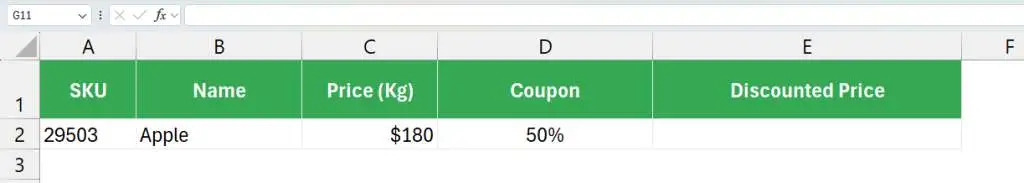
We will use our custom DISCOUNTEDPRICE function in this case. Refer to the following GIF.
Let us assume that the discount does not apply to the same product. So, we will keep the corresponding cell blank.


In this case, as we don’t have the discount, we will not specify it within our custom DISCOUNTEDPRICE function. Refer to the following GIF.
Syntax
The ISOMITTED is a simple function with the following syntax. It is combined with the LAMBDA and IF functions to create a custom function in Excel.
=ISOMITTED(argument)Where the argument needs to be replaced with the LAMBDA function argument to be tested if missing or not.
Important Notes:
- Omitting an argument is not the same as passing a blank value.
- It needs to be combined with the IF function to get the default values when the given argument is not specified.
How to use the ISOMITTED Function in Excel
Download the example spreadsheet used to demonstrate the ISOMITTED function in the upcoming section. Practice is the key to success!
Task
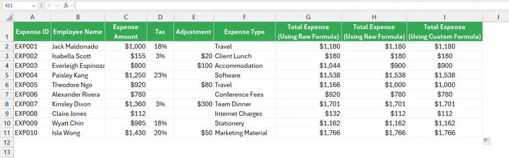
Suppose that you are a Senior Accountant who wishes to create a custom function to calculate total reimbursement based on the following things:
- Expense Amount
- Applicable Tax
- Special Adjustment
Refer to the following image:
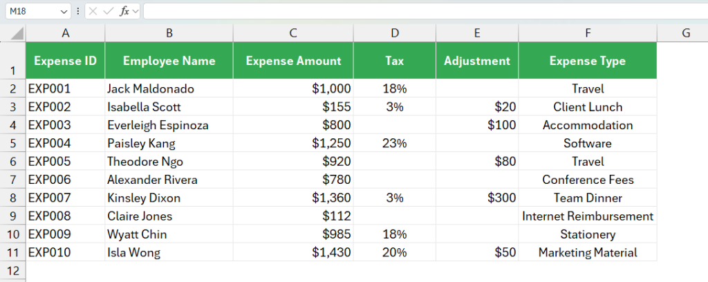
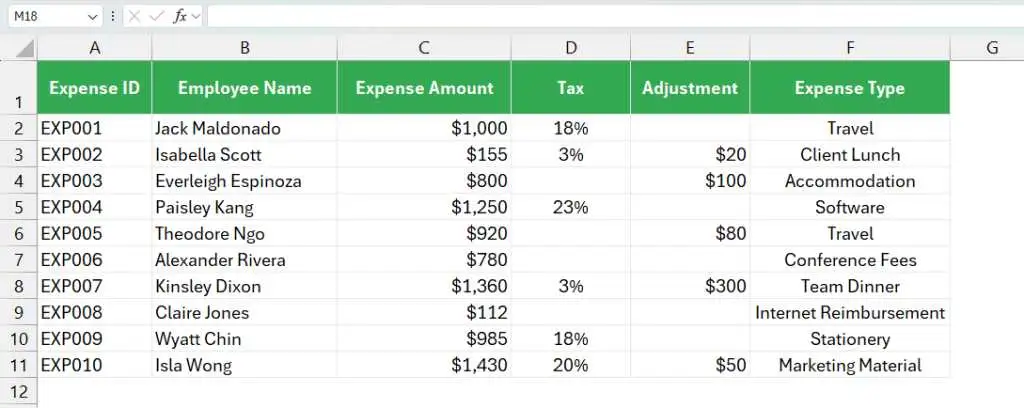
The problem here is that both the tax and special adjustments are variables. Sometimes they are not mentioned in the above table.
That’s why we need to make the following assumptions in our formula:
- If the tax is not mentioned, the default value will be 18%
- If the adjustment is not mentioned, the default value will be 0 (zero)
It means that these two values will be optional in our custom formula. If the user will not enter them, the default values will be passed.
STEP 1: Build your formula
In this step, we will create a formula using built-in functions in Excel to calculate the total reimbursement. We will consider the conditions as discussed above.
Our formula would be as follows:
=C2 + (C2 * IF(ISOMITTED(D2), 0.18, D2)) + IF(ISOMITTED(E2), 0, E2)Where,
- C2 is the cell that holds the first expense.
- (C2 * IF(ISOMITTED(D2), 0.18, D2)) is the formula to calculate the tax amount.
- IF(ISOMITTED(D2), 0.18, D2) is the formula to determine whether the tax is mentioned. If the tax is not mentioned, it returns 18% as the default value.
- IF(ISOMITTED(E2), 0, E2) is the formula for determining whether the adjustment is mentioned. If it is not, it returns 0 (zero) as the default value.
If we put the above formula in column G, we will get the total reimbursement amount as shown below.
STEP 2: Build the LAMBDA version of the formula
The LAMBDA function requires parameters and a calculation. We already created a formula (calculation) in the previous section. Now, let us get the parameters.
- amount – It is the parameter representing the expense amount
- tax – It is the parameter representing the applicable tax amount
- adjustment – It is the parameter representing the adjustment amount
Our Lambda version of the formula will be:
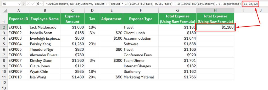
=LAMBDA(amount, tax, adjustment, amount + (amount * IF(ISOMITTED(tax), 0.18, tax)) + IF(ISOMITTED(adjustment), 0, adjustment))We will get an error if we put this formula as is in column H.


This error is caused by the function’s inability to find the parameters. The solution is to add the cell references to the formula, as shown below.
=LAMBDA(amount,tax,adjustment, amount + (amount * IF(ISOMITTED(tax), 0.18, tax)) + IF(ISOMITTED(adjustment), 0, adjustment))(C2, D2, E2)Now, it works fine.

Note that you can leverage the LET function in Excel to name the calculation results within the formula. It will help us easily understand each part of the formula.
=LAMBDA(amount, tax, adjustment,
        LET(
            t, IF(ISOMITTED(tax), 0.18, tax),
            a, IF(ISOMITTED(adjustment), 0, adjustment),
            amount + (amount * t) + a
        )
)(C2, D2, E2)
STEP 3: Create a Custom Function
In this step, we will name our LAMBDA version of the formula. We will reuse that name to calculate the total reimbursement amount within a few seconds.
- Go to Formulas from the ribbon
- In the Defined Names section
- Click on the Name Manager icon
- A dialog box will appear on your screen as shown in the following image
- Click the New button
- A new popup will appear
- Put a desired name in the Name box as shown below
(I have put “REIMBURSEMENT”) - Make sure that the scope is set to Workbook
- Copy and paste the LAMBDA version of the formula in the Refers to box as follows
- Click the OK button to close the popup
- You will be redirected to the Name Manager dialog box
- Click the Close button


Important Notes:
- The name can be a maximum of 255 characters long
- It must start with the letter (A-Z, a-z) or an underscore (_)
- Function names do not contain spaces or special characters like @, !, #, $, %, etc.
- Make sure to choose a unique name to avoid potential conflict with the existing functions
- Avoid using cell references like A1, B1, D2, R100, etc. in your custom name
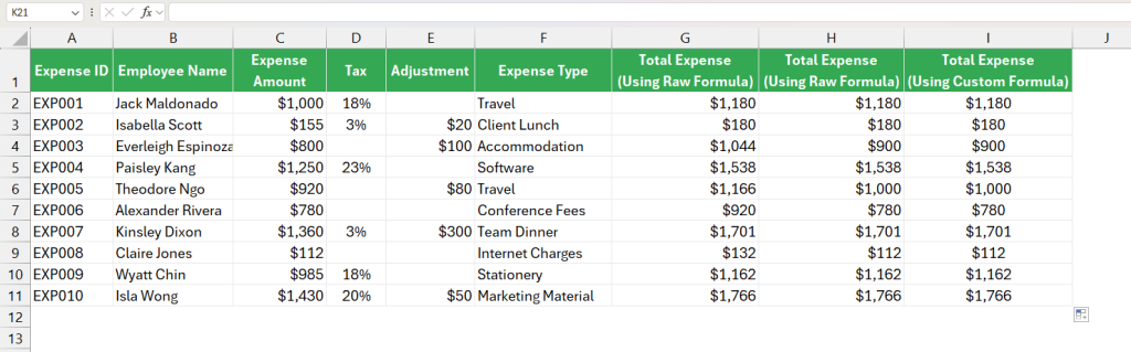
STEP 4: Use your Custom Function
Using your custom formula is pretty straightforward. The process is similar to using a pre-built function in Excel.
Here are the steps,
- Select the desired cell
- Type =REIMBURSEMENT
- Choose the first option from the popup
- Enter the parameters
(In this case, parameters act as arguments in prebuilt functions) - Close the brackets using )
- Hit Enter


The results are displayed in the following image.
How to use the Custom function with optional arguments
Let us discuss how we can benefit from using the ISOMITTED within the LAMBDA function.
Scenario #1
Suppose that you wish to calculate the reimbursement with the following conditions:
- Expense amount: $1000
- Tax: 20%
- Adjustment: $300
Now, let’s use our custom function named the REIMBURSEMENT to calculate the total:
Scenario #2
Next, let us assume another scenario where we have an expense and an adjustment amount only, without the tax mentioned.
- Expense amount: $1000
- Adjustment: $300
Refer to the following GIF.

In the above calculation, the formula has passed the default tax value: 18%. That’s why the total reimbursement is only $1480.
Scenario #3
Finally, let us assume that only the expense amount ($1000) is mentioned. We don’t have the tax and adjustment. Refer to the following GIF.
Please take note that using the , is compulsory when you wish to skip an optional argument of the custom formula created using the LAMBDA and ISOMITTED function.
Takeaway
Learning the ISOMITTED function is a critical step when you are creating a custom formula in Excel. Make sure to use the , properly while using your custom function and skipping the optional arguments.
To learn more about the LAMBDA function in Excel, click here.
I hope this article taught you all the bells and whistles of the ISOMITTED function. Please comment below if you are stuck or encounter any particular error while using it. I will answer your questions as soon as possible.
Additional Resources:
- Learn All Excel Information Functions (With Examples)
- LAMBDA Function in Excel
- MAP Function in Excel
- IF Function in Excel
Get an Office 365 Subscription to Access all the powerful Functions and Tools in Excel.